Amounts and proportions
When you visualize proportions with ggplot, you’ll typically go through a two-step process:
- Summarize the data with dplyr (typically with a combination of
group_by()andsummarize()) - Plot the summarized data
Manipulating data with dplyr
You had some experience with dplyr functions in the RStudio primers, but we’ll briefly review them here.
There are 6 important verbs that you’ll typically use when working with data:
- Extract rows/cases with
filter() - Extract columns/variables with
select() - Arrange/sort rows with
arrange() - Make new columns/variables with
mutate() - Make group summaries with
group_by %>% summarize()
Every dplyr verb follows the same pattern. The first argument is always a data frame, and the function always returns a data frame:
VERB(DATA_TO_TRANSFORM, STUFF_IT_DOES)Filtering with filter()
The filter() function takes two arguments: a data frame to transform, and a set of tests. It will return each row for which the test is TRUE.
This code, for instance, will look at the gapminder dataset and return all rows where country is equal to “Denmark”:
filter(gapminder, country == "Denmark")
## # A tibble: 12 x 6
##    country continent  year lifeExp     pop gdpPercap
##    <fct>   <fct>     <int>   <dbl>   <int>     <dbl>
##  1 Denmark Europe     1952    70.8 4334000     9692.
##  2 Denmark Europe     1957    71.8 4487831    11100.
##  3 Denmark Europe     1962    72.4 4646899    13583.
##  4 Denmark Europe     1967    73.0 4838800    15937.
##  5 Denmark Europe     1972    73.5 4991596    18866.
##  6 Denmark Europe     1977    74.7 5088419    20423.
##  7 Denmark Europe     1982    74.6 5117810    21688.
##  8 Denmark Europe     1987    74.8 5127024    25116.
##  9 Denmark Europe     1992    75.3 5171393    26407.
## 10 Denmark Europe     1997    76.1 5283663    29804.
## 11 Denmark Europe     2002    77.2 5374693    32167.
## 12 Denmark Europe     2007    78.3 5468120    35278.
Notice that there are two equal signs (==). This is because it’s a logical test, similar to greater than (>) or less than (<). When you use a single equal sign, you set an argument (like data = gapminder); when you use two, you are doing a test. There are lots of different ways to do logical tests:
| Test | Meaning |
|---|---|
x < y |
Less than |
x > y |
Greater than |
x == y |
Equal to |
x <= y |
Less than or equal to |
x >= y |
Greater than or equal to |
x != y |
Not equal to |
x %in% y |
In (group membership) |
is.na(x) |
Is missing |
!is.na(x) |
Is not missing |
Your turn: Use filter() and logical tests to show:
- The data for Canada
- All data for countries in Oceania
- Rows where life expectancy is greater than 82
You can also use multiple conditions, and these will extract rows that meet every test. By default, if you separate the tests with a comma, R will consider this an “and” test and find rows that are both Denmark and greater than 2000.
filter(gapminder, country == "Denmark", year > 2000)
## # A tibble: 2 x 6
##   country continent  year lifeExp     pop gdpPercap
##   <fct>   <fct>     <int>   <dbl>   <int>     <dbl>
## 1 Denmark Europe     2002    77.2 5374693    32167.
## 2 Denmark Europe     2007    78.3 5468120    35278.
You can also use “or” with “|” and “not” with “!”:
| Operator | Meaning |
|---|---|
a & b |
and |
a | b |
or |
!a |
not |
Your turn: Use filter() and logical tests to show:
- Canada before 1970
- Countries where life expectancy in 2007 is below 50
- Countries where life expectancy in 2007 is below 50 and are not in Africa
Beware of some common mistakes! You can’t collapse multiple tests into one. Instead, use two separate tests:
# This won't work!
filter(gapminder, 1960 < year < 1980)

# This will work
filter(gapminder, 1960 < year, year < 1980)
Also, you can avoid stringing together lots of tests by using the %in% operator, which checks to see if a value is in a list of values.
# This works, but is tedious
filter(gapminder,
       country == "Mexico" | country == "Canada" | country == "United States")

# This is more concise and easier to add other countries later
filter(gapminder,
       country %in% c("Mexico", "Canada", "United States"))
Adding new columns with mutate()
You create new columns with the mutate() function. You can create a single column like this:
mutate(gapminder, gdp = gdpPercap * pop)
## # A tibble: 1,704 x 7
##    country     continent  year lifeExp      pop gdpPercap          gdp
##    <fct>       <fct>     <int>   <dbl>    <int>     <dbl>        <dbl>
##  1 Afghanistan Asia       1952    28.8  8425333      779.  6567086330.
##  2 Afghanistan Asia       1957    30.3  9240934      821.  7585448670.
##  3 Afghanistan Asia       1962    32.0 10267083      853.  8758855797.
##  4 Afghanistan Asia       1967    34.0 11537966      836.  9648014150.
##  5 Afghanistan Asia       1972    36.1 13079460      740.  9678553274.
##  6 Afghanistan Asia       1977    38.4 14880372      786. 11697659231.
##  7 Afghanistan Asia       1982    39.9 12881816      978. 12598563401.
##  8 Afghanistan Asia       1987    40.8 13867957      852. 11820990309.
##  9 Afghanistan Asia       1992    41.7 16317921      649. 10595901589.
## 10 Afghanistan Asia       1997    41.8 22227415      635. 14121995875.
## # … with 1,694 more rows
And you can create multiple columns by including a comma-separated list of new columns to create:
mutate(gapminder, gdp = gdpPercap * pop,
                  pop_mill = round(pop / 1000000))
## # A tibble: 1,704 x 8
##    country     continent  year lifeExp      pop gdpPercap          gdp pop_mill
##    <fct>       <fct>     <int>   <dbl>    <int>     <dbl>        <dbl>    <dbl>
##  1 Afghanistan Asia       1952    28.8  8425333      779.  6567086330.        8
##  2 Afghanistan Asia       1957    30.3  9240934      821.  7585448670.        9
##  3 Afghanistan Asia       1962    32.0 10267083      853.  8758855797.       10
##  4 Afghanistan Asia       1967    34.0 11537966      836.  9648014150.       12
##  5 Afghanistan Asia       1972    36.1 13079460      740.  9678553274.       13
##  6 Afghanistan Asia       1977    38.4 14880372      786. 11697659231.       15
##  7 Afghanistan Asia       1982    39.9 12881816      978. 12598563401.       13
##  8 Afghanistan Asia       1987    40.8 13867957      852. 11820990309.       14
##  9 Afghanistan Asia       1992    41.7 16317921      649. 10595901589.       16
## 10 Afghanistan Asia       1997    41.8 22227415      635. 14121995875.       22
## # … with 1,694 more rows
You can also do conditional tests within mutate() using the ifelse() function. This works like the =IFELSE function in Excel. Feed the function three arguments: (1) a test, (2) the value if the test is true, and (3) the value if the test is false:
ifelse(TEST, VALUE_IF_TRUE, VALUE_IF_FALSE)We can create a new column that is a binary indicator for whether the country’s row is after 1960:
mutate(gapminder, after_1960 = ifelse(year > 1960, TRUE, FALSE))
## # A tibble: 1,704 x 7
##    country     continent  year lifeExp      pop gdpPercap after_1960
##    <fct>       <fct>     <int>   <dbl>    <int>     <dbl> <lgl>
##  1 Afghanistan Asia       1952    28.8  8425333      779. FALSE
##  2 Afghanistan Asia       1957    30.3  9240934      821. FALSE
##  3 Afghanistan Asia       1962    32.0 10267083      853. TRUE
##  4 Afghanistan Asia       1967    34.0 11537966      836. TRUE
##  5 Afghanistan Asia       1972    36.1 13079460      740. TRUE
##  6 Afghanistan Asia       1977    38.4 14880372      786. TRUE
##  7 Afghanistan Asia       1982    39.9 12881816      978. TRUE
##  8 Afghanistan Asia       1987    40.8 13867957      852. TRUE
##  9 Afghanistan Asia       1992    41.7 16317921      649. TRUE
## 10 Afghanistan Asia       1997    41.8 22227415      635. TRUE
## # … with 1,694 more rows
We can also use text labels instead of TRUE and FALSE:
mutate(gapminder,
       after_1960 = ifelse(year > 1960, "After 1960", "Before 1960"))
## # A tibble: 1,704 x 7
##    country     continent  year lifeExp      pop gdpPercap after_1960
##    <fct>       <fct>     <int>   <dbl>    <int>     <dbl> <chr>
##  1 Afghanistan Asia       1952    28.8  8425333      779. Before 1960
##  2 Afghanistan Asia       1957    30.3  9240934      821. Before 1960
##  3 Afghanistan Asia       1962    32.0 10267083      853. After 1960
##  4 Afghanistan Asia       1967    34.0 11537966      836. After 1960
##  5 Afghanistan Asia       1972    36.1 13079460      740. After 1960
##  6 Afghanistan Asia       1977    38.4 14880372      786. After 1960
##  7 Afghanistan Asia       1982    39.9 12881816      978. After 1960
##  8 Afghanistan Asia       1987    40.8 13867957      852. After 1960
##  9 Afghanistan Asia       1992    41.7 16317921      649. After 1960
## 10 Afghanistan Asia       1997    41.8 22227415      635. After 1960
## # … with 1,694 more rows
Your turn: Use mutate() to:
- Add an
africacolumn that is TRUE if the country is on the African continent - Add a column for logged GDP per capita
- Add an
africa_asiacolumn that says “Africa or Asia” if the country is in Africa or Asia, and “Not Africa or Asia” if it’s not
Combining multiple verbs with pipes (%>%)
What if you want to filter to include only rows from 2002 and make a new column with the logged GDP per capita? Doing this requires both filter() and mutate(), so we need to find a way to use both at once.
One solution is to use intermediate variables for each step:
gapminder_2002_filtered <- filter(gapminder, year == 2002)

gapminder_2002_logged <- mutate(gapminder_2002_filtered, log_gdpPercap = log(gdpPercap))
That works fine, but your environment panel will start getting full of lots of intermediate data frames.
Another solution is to nest the functions inside each other. Remember that all dplyr functions return data frames, so you can feed the results of one into another:
filter(mutate(gapminder, log_gdpPercap = log(gdpPercap)),
       year == 2002)
That works too, but it gets really complicated once you have even more functions, and it’s hard to keep track of which function’s arguments go where. I’d avoid doing this entirely.
One really nice solution is to use a pipe, or %>%. The pipe takes an object on the left and passes it as the first argument of the function on the right.
# gapminder will automatically get placed in the _____ spot
gapminder %>% filter(_____, country == "Canada")
These two lines of code do the same thing:
filter(gapminder, country == "Canada")

gapminder %>% filter(country == "Canada")
Using pipes, you can start with a data frame, pass it to one verb, then pass the output of that verb to the next verb, and so on. When reading any code with a %>%, it’s easiest to read the %>% as “and then”. This would read:
Take the
gapminderdataset and then filter it so that it only has rows from 2002 and then add a new column with the logged GDP per capita
gapminder %>%
  filter(year == 2002) %>%
  mutate(log_gdpPercap = log(gdpPercap))
Here’s another way to think about pipes more conceptually. This isn’t valid R code, obviously, but imagine you’re going to take yourself, and then wake up, get out of bed, get dressed, and leave the house. Writing that whole process as nested functions would look like this:
leave_house(get_dressed(get_out_of_bed(wake_up(me, time = "8:00"), side = "correct"), pants = TRUE, shirt = TRUE), car = TRUE, bike = FALSE)Instead of nesting everything, we can use pipes to chain these together. This would read
Take myself, and then wake up at 8:00, and then get out of bed on the correct side, and then get dressed with pants and a shirt, and then leave the house in a car
me %>%
  wake_up(time = "8:00") %>%
  get_out_of_bed(side = "correct") %>%
  get_dressed(pants = TRUE, shirt = TRUE) %>%
  leave_house(car = TRUE, bike = FALSE)
Summarizing data by groups with group_by() %>% summarize()
The summarize() verb takes an entire frame and calculates summary information about it. For instance, this will find the average life expectancy for the whole gapminder data:
gapminder %>% summarize(mean_life = mean(lifeExp))
## # A tibble: 1 x 1
##   mean_life
##       <dbl>
## 1      59.5
You can also make multiple summary variables, just like mutate(), and it will return a column for each:
gapminder %>% summarize(mean_life = mean(lifeExp),
                        min_life = min(lifeExp))
## # A tibble: 1 x 2
##   mean_life min_life
##       <dbl>    <dbl>
## 1      59.5     23.6
Your turn: Use summarize() to calculate:
- The first (minimum) year in the
gapminderdataset - The last (maximum) year in the dataset
- The number of rows in the dataset (use the dplyr cheatsheet)
- The number of distinct countries in the dataset (use the dplyr cheatsheet)
Your turn: Use filter() and summarize() to calculate the median life expectancy on the African continent in 2007:
Notice that summarize() on its own summarizes the whole dataset, so you only get a single row back. These values are the averages and minimums for the entire data frame. If you group your data into separate subgroups, you can use summarize() to calculate summary statistics for each group. Do this with group_by().
The group_by() function puts rows into groups based on values in a column. If you run this:
gapminder %>% group_by(continent)
## # A tibble: 1,704 x 6
## # Groups:   continent [5]
##    country     continent  year lifeExp      pop gdpPercap
##    <fct>       <fct>     <int>   <dbl>    <int>     <dbl>
##  1 Afghanistan Asia       1952    28.8  8425333      779.
##  2 Afghanistan Asia       1957    30.3  9240934      821.
##  3 Afghanistan Asia       1962    32.0 10267083      853.
##  4 Afghanistan Asia       1967    34.0 11537966      836.
##  5 Afghanistan Asia       1972    36.1 13079460      740.
##  6 Afghanistan Asia       1977    38.4 14880372      786.
##  7 Afghanistan Asia       1982    39.9 12881816      978.
##  8 Afghanistan Asia       1987    40.8 13867957      852.
##  9 Afghanistan Asia       1992    41.7 16317921      649.
## 10 Afghanistan Asia       1997    41.8 22227415      635.
## # … with 1,694 more rows
…you won’t see anything different! R has put the dataset into separate invisible groups behind the scenes, but you haven’t done anything with those groups, so nothing has really happened. If you do things with those groups with summarize(), though, group_by() becomes much more useful.
For instance, this will take the gapminder data frame, group it by continent, and then summarize it by calculating the number of distinct countries in each group. It will return one row for each group, so there should be a row for each continent:
gapminder %>%
  group_by(continent) %>%
  summarize(n_countries = n_distinct(country))
## # A tibble: 5 x 2
## continent n_countries
## <fct> <int>
## 1 Africa 52
## 2 Americas 25
## 3 Asia 33
## 4 Europe 30
## 5 Oceania 2You can calculate multiple summary statistics, as before:
gapminder %>%
  group_by(continent) %>%
  summarize(n_countries = n_distinct(country),
            avg_life_exp = mean(lifeExp))
## # A tibble: 5 x 3
## continent n_countries avg_life_exp
## <fct> <int> <dbl>
## 1 Africa 52 48.9
## 2 Americas 25 64.7
## 3 Asia 33 60.1
## 4 Europe 30 71.9
## 5 Oceania 2 74.3Your turn: Find the minimum, maximum, and median life expectancy for each continent:
Your turn: Find the minimum, maximum, and median life expectancy for each continent in 2007 only:
Finally, you can group by multiple columns and R will create subgroups for every combination of the groups and return the number of rows of combinations. For instance, we can calculate the average life expectancy by both year and continent and we’ll get 60 rows, since there are 5 continents and 12 years (5 × 12 = 60):
gapminder %>%
  group_by(continent, year) %>%
  summarize(avg_life_exp = mean(lifeExp))
## # A tibble: 60 x 3
## # Groups: continent [5]
## continent year avg_life_exp
## <fct> <int> <dbl>
## 1 Africa 1952 39.1
## 2 Africa 1957 41.3
## 3 Africa 1962 43.3
## 4 Africa 1967 45.3
## 5 Africa 1972 47.5
## 6 Africa 1977 49.6
## 7 Africa 1982 51.6
## 8 Africa 1987 53.3
## 9 Africa 1992 53.6
## 10 Africa 1997 53.6
## # … with 50 more rowsSelecting with select()
The last two verbs are far simpler than filter(), mutate(), and group_by() %>% summarize().
You can choose specific columns with the select() verb. This will only keep two columns: lifeExp and year:
gapminder %>% select(lifeExp, year)
## # A tibble: 1,704 x 2
##    lifeExp  year
##      <dbl> <int>
##  1    28.8  1952
##  2    30.3  1957
##  3    32.0  1962
##  4    34.0  1967
##  5    36.1  1972
##  6    38.4  1977
##  7    39.9  1982
##  8    40.8  1987
##  9    41.7  1992
## 10    41.8  1997
## # … with 1,694 more rows
You can remove specific columns by prefacing the column names with -, like -lifeExp:
gapminder %>% select(-lifeExp)
## # A tibble: 1,704 x 5
##    country     continent  year      pop gdpPercap
##    <fct>       <fct>     <int>    <int>     <dbl>
##  1 Afghanistan Asia       1952  8425333      779.
##  2 Afghanistan Asia       1957  9240934      821.
##  3 Afghanistan Asia       1962 10267083      853.
##  4 Afghanistan Asia       1967 11537966      836.
##  5 Afghanistan Asia       1972 13079460      740.
##  6 Afghanistan Asia       1977 14880372      786.
##  7 Afghanistan Asia       1982 12881816      978.
##  8 Afghanistan Asia       1987 13867957      852.
##  9 Afghanistan Asia       1992 16317921      649.
## 10 Afghanistan Asia       1997 22227415      635.
## # … with 1,694 more rows
You can also rename columns using select(). Follow this pattern: select(old_name = new_name).
gapminder %>% select(year, country, life_expectancy = lifeExp)
## # A tibble: 1,704 x 3
##     year country     life_expectancy
##    <int> <fct>                 <dbl>
##  1  1952 Afghanistan            28.8
##  2  1957 Afghanistan            30.3
##  3  1962 Afghanistan            32.0
##  4  1967 Afghanistan            34.0
##  5  1972 Afghanistan            36.1
##  6  1977 Afghanistan            38.4
##  7  1982 Afghanistan            39.9
##  8  1987 Afghanistan            40.8
##  9  1992 Afghanistan            41.7
## 10  1997 Afghanistan            41.8
## # … with 1,694 more rows
Alternatively, there’s a special rename() verb that will, um, rename, while keeping all the other columns:
gapminder %>% rename(life_expectancy = lifeExp)
## # A tibble: 1,704 x 6
##    country     continent  year life_expectancy      pop gdpPercap
##    <fct>       <fct>     <int>           <dbl>    <int>     <dbl>
##  1 Afghanistan Asia       1952            28.8  8425333      779.
##  2 Afghanistan Asia       1957            30.3  9240934      821.
##  3 Afghanistan Asia       1962            32.0 10267083      853.
##  4 Afghanistan Asia       1967            34.0 11537966      836.
##  5 Afghanistan Asia       1972            36.1 13079460      740.
##  6 Afghanistan Asia       1977            38.4 14880372      786.
##  7 Afghanistan Asia       1982            39.9 12881816      978.
##  8 Afghanistan Asia       1987            40.8 13867957      852.
##  9 Afghanistan Asia       1992            41.7 16317921      649.
## 10 Afghanistan Asia       1997            41.8 22227415      635.
## # … with 1,694 more rows
Arranging data with arrange()
The arrange() verb sorts data. By default it sorts ascendingly, putting the lowest values first:
gapminder %>% arrange(lifeExp)
## # A tibble: 1,704 x 6
##    country      continent  year lifeExp     pop gdpPercap
##    <fct>        <fct>     <int>   <dbl>   <int>     <dbl>
##  1 Rwanda       Africa     1992    23.6 7290203      737.
##  2 Afghanistan  Asia       1952    28.8 8425333      779.
##  3 Gambia       Africa     1952    30    284320      485.
##  4 Angola       Africa     1952    30.0 4232095     3521.
##  5 Sierra Leone Africa     1952    30.3 2143249      880.
##  6 Afghanistan  Asia       1957    30.3 9240934      821.
##  7 Cambodia     Asia       1977    31.2 6978607      525.
##  8 Mozambique   Africa     1952    31.3 6446316      469.
##  9 Sierra Leone Africa     1957    31.6 2295678     1004.
## 10 Burkina Faso Africa     1952    32.0 4469979      543.
## # … with 1,694 more rows
You can reverse that by wrapping the column name with desc():
gapminder %>% arrange(desc(lifeExp))
## # A tibble: 1,704 x 6
##    country          continent  year lifeExp       pop gdpPercap
##    <fct>            <fct>     <int>   <dbl>     <int>     <dbl>
##  1 Japan            Asia       2007    82.6 127467972    31656.
##  2 Hong Kong, China Asia       2007    82.2   6980412    39725.
##  3 Japan            Asia       2002    82   127065841    28605.
##  4 Iceland          Europe     2007    81.8    301931    36181.
##  5 Switzerland      Europe     2007    81.7   7554661    37506.
##  6 Hong Kong, China Asia       2002    81.5   6762476    30209.
##  7 Australia        Oceania    2007    81.2  20434176    34435.
##  8 Spain            Europe     2007    80.9  40448191    28821.
##  9 Sweden           Europe     2007    80.9   9031088    33860.
## 10 Israel           Asia       2007    80.7   6426679    25523.
## # … with 1,694 more rows
You can sort by multiple columns by specifying them in a comma separated list. For example, we can sort by continent and then sort by life expectancy within the continents:
gapminder %>%
  arrange(continent, desc(lifeExp))
## # A tibble: 1,704 x 6
##    country   continent  year lifeExp      pop gdpPercap
##    <fct>     <fct>     <int>   <dbl>    <int>     <dbl>
##  1 Reunion   Africa     2007    76.4   798094     7670.
##  2 Reunion   Africa     2002    75.7   743981     6316.
##  3 Reunion   Africa     1997    74.8   684810     6072.
##  4 Libya     Africa     2007    74.0  6036914    12057.
##  5 Tunisia   Africa     2007    73.9 10276158     7093.
##  6 Reunion   Africa     1992    73.6   622191     6101.
##  7 Tunisia   Africa     2002    73.0  9770575     5723.
##  8 Mauritius Africa     2007    72.8  1250882    10957.
##  9 Libya     Africa     2002    72.7  5368585     9535.
## 10 Algeria   Africa     2007    72.3 33333216     6223.
## # … with 1,694 more rows
That’s it!
Those are the main verbs you’ll deal with in this class. There are dozens of other really useful ones—check out the dplyr and tidyr cheat sheet for examples.
Changing colors, shapes, and sizes, with scale_*()
Recall from session 3 that the grammar of graphics uses a set of layers to define elements of plots:

In tomorrow’s session, you’ll learn all about the Theme layer. Here we’ll briefly cover the Scales layer, which we use for changing aspects of the different aesthetics, like using logged axes or changing colors or shapes.
All the functions that deal with scales conveniently follow the same naming pattern:
scale_AESTHETIC_DETAILS()Here are some common scale functions:
scale_x_continuous()
scale_y_reverse()
scale_color_viridis_c()
scale_shape_manual(values = c(19, 13, 15))
scale_fill_manual(values = c("red", "orange", "blue"))
You can see a list of all of the possible scale functions here, and you should reference that documentation (and the excellent examples) often when working with these functions.
As long as you have mapped a variable to an aesthetic with aes(), you can use the scale_*() functions to deal with it. For instance, in this ggplot, we have mapped variables to x, y, and fill, which means we can use those corresponding scale functions to manipulate how those aesthetics are shown. Here we reverse the y-axis (ew, don’t really do this), and we use a discrete viridis color palette:
continent_counts <- gapminder %>%
  group_by(continent) %>%
  summarize(countries = n_distinct(country))

ggplot(continent_counts, aes(x = continent, y = countries, fill = continent)) +
  geom_col() +
  scale_y_reverse() +  # lol this is bad; don't do it in real life
  scale_fill_viridis_d()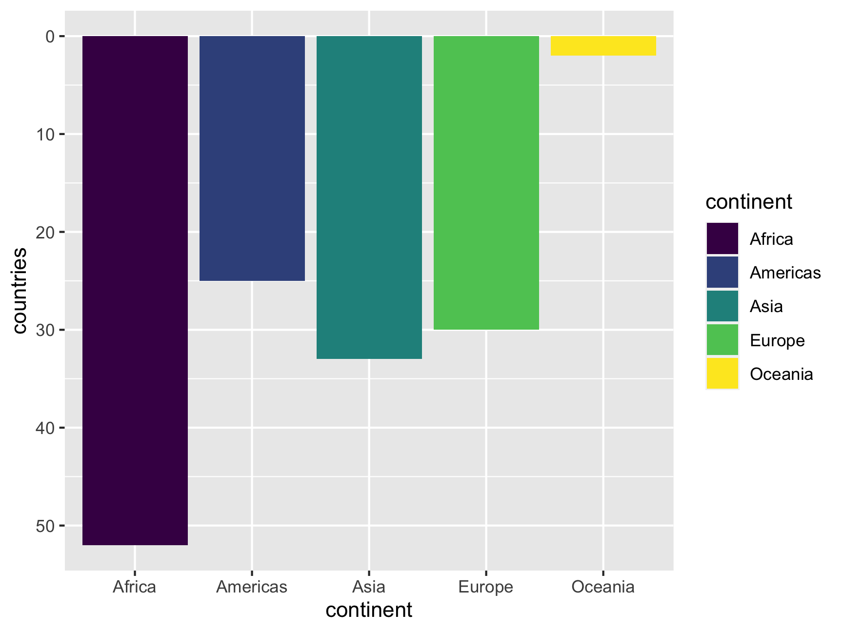
You can also use different arguments in the scale functions—again, check the documentation for examples. For instance, if we want to use the plasma palette from the viridis package, we can set that as an option:
ggplot(continent_counts, aes(x = continent, y = countries, fill = continent)) +
  geom_col() +
  scale_fill_viridis_d(option = "plasma")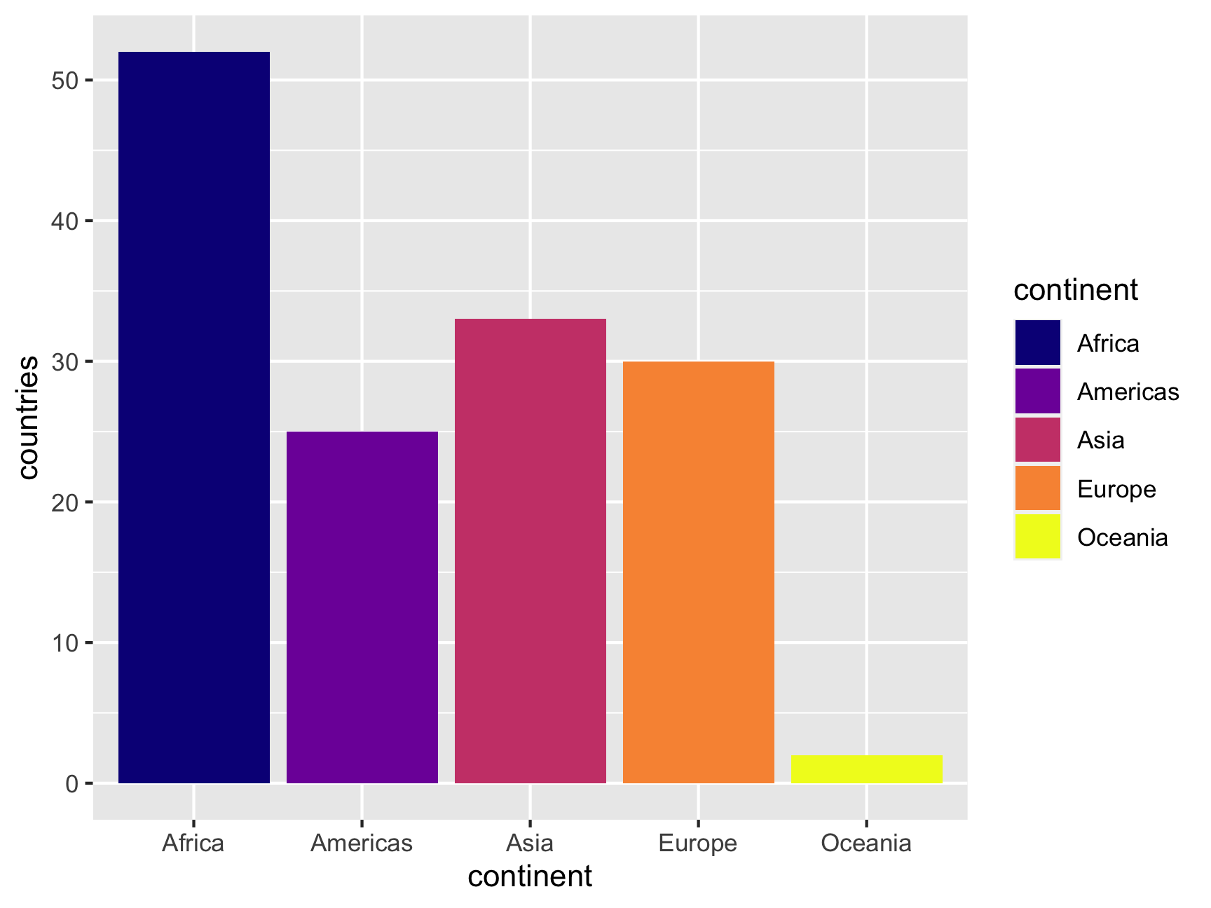
That yellow might be too bright and hard to see, so we can tell ggplot to not use the full range of the palette, ending at 90% of the range instead:
ggplot(continent_counts, aes(x = continent, y = countries, fill = continent)) +
  geom_col() +
  scale_fill_viridis_d(option = "plasma", end = 0.9)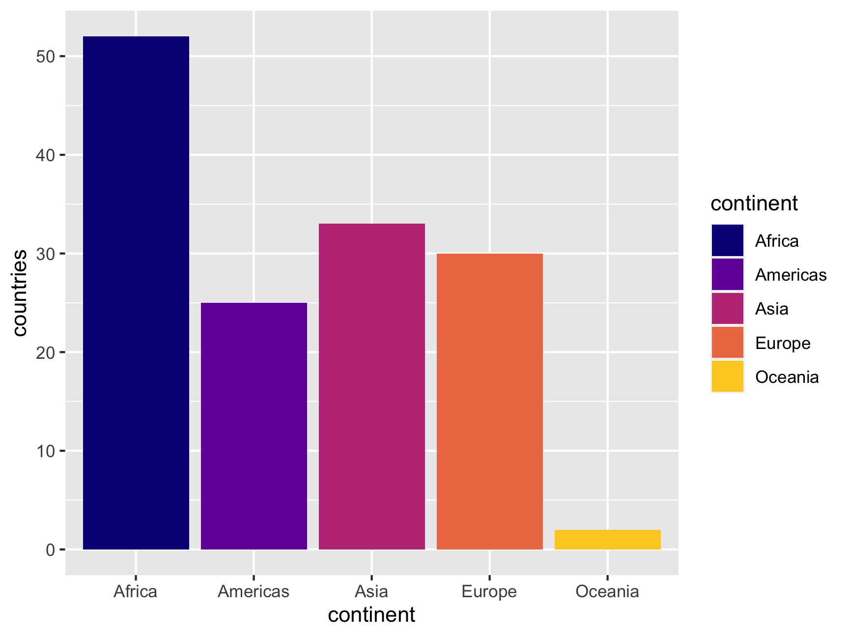
Instead of letting R calculate the colors from a general palette, you can also specify your own colors with scale_fill_manual() and feeding it a list of values—generally as hex codes or a name from a list of built-in R colors:
ggplot(continent_counts, aes(x = continent, y = countries, fill = continent)) +
  geom_col() +
  scale_fill_manual(values = c("chartreuse4", "cornsilk4", "black", "#fc03b6", "#5c47d6"))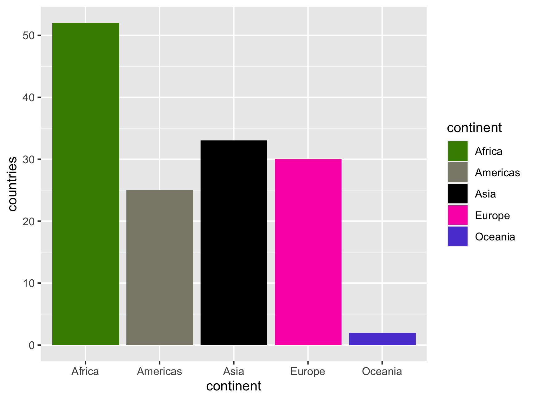
Scale functions also work for other aesthetics like shape or color or size. For instance, consider this plot, which has all three:
gapminder_2007 <- gapminder %>%
  filter(year == 2007)

ggplot(gapminder_2007,
       aes(x = gdpPercap, y = lifeExp,
           color = continent, shape = continent, size = pop)) +
  geom_point() +
  scale_x_log10()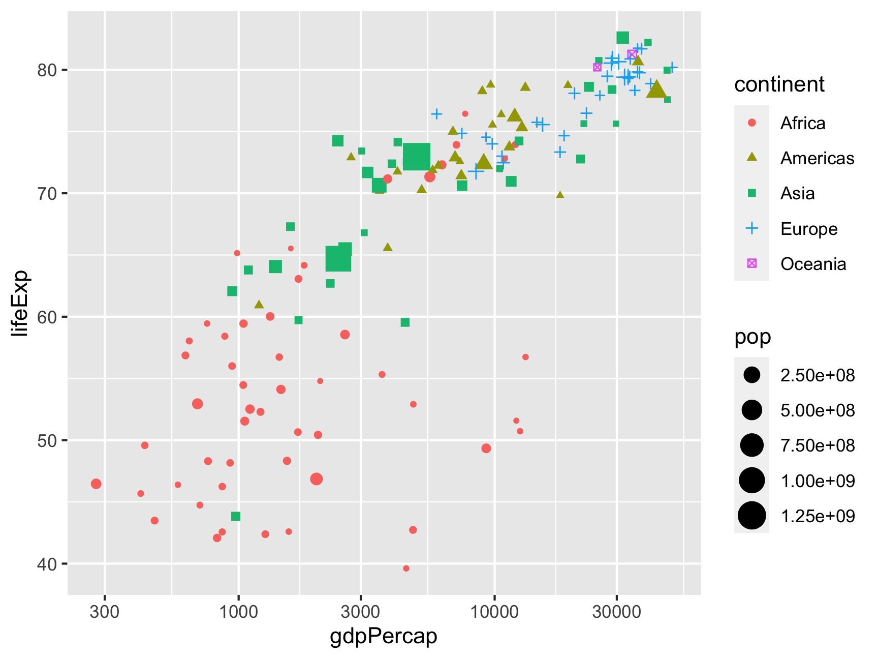
We can change the colors of the points with scale_color_*():
ggplot(gapminder_2007,
       aes(x = gdpPercap, y = lifeExp,
           color = continent, shape = continent, size = pop)) +
  geom_point() +
  scale_x_log10() +
  scale_color_manual(values = c("chartreuse4", "cornsilk4", "black", "#fc03b6", "#5c47d6"))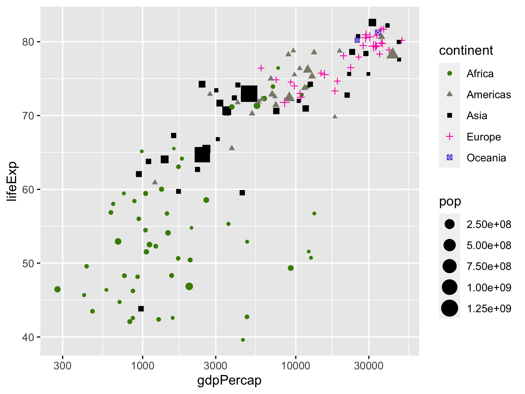
We can change the shapes with scale_shape_*(). If you run ?pch in your console or search for pch in the help, you can see all the possible shapes.
ggplot(gapminder_2007,
       aes(x = gdpPercap, y = lifeExp,
           color = continent, shape = continent, size = pop)) +
  geom_point() +
  scale_x_log10() +
  scale_shape_manual(values = c(12, 9, 17, 19, 15))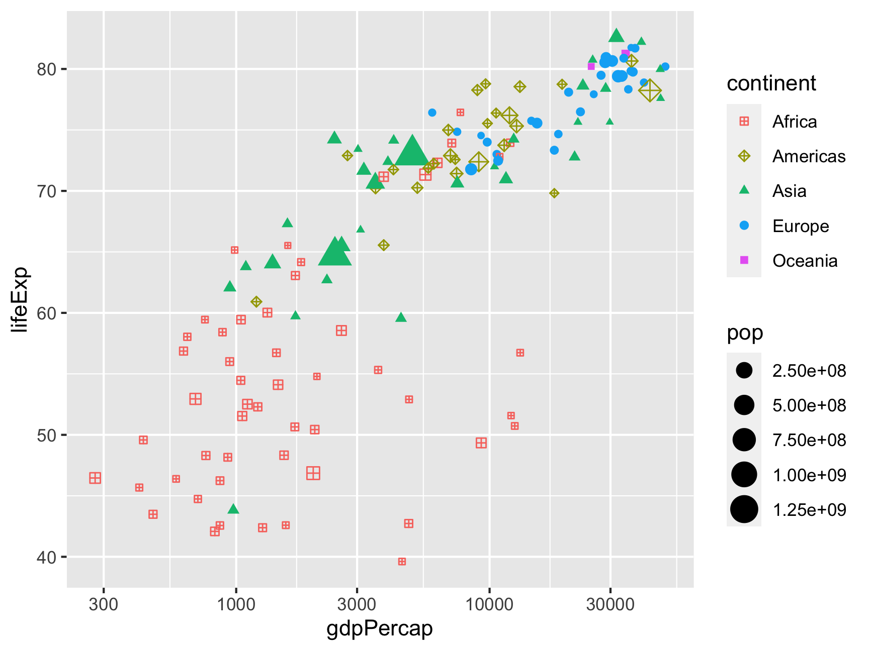
You can change the size with scale_size_*(). Here we make it so the smallest possible size is 1 and the largest is 15:
ggplot(gapminder_2007,
       aes(x = gdpPercap, y = lifeExp,
           color = continent, shape = continent, size = pop)) +
  geom_point() +
  scale_x_log10() +
  scale_size_continuous(range = c(1, 15))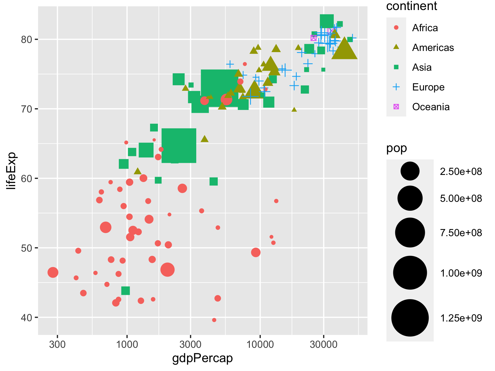
We can even do all three at once:
ggplot(gapminder_2007,
       aes(x = gdpPercap, y = lifeExp,
           color = continent, shape = continent, size = pop)) +
  geom_point() +
  scale_x_log10() +
  scale_color_manual(values = c("chartreuse4", "cornsilk4", "black", "#fc03b6", "#5c47d6")) +
  scale_shape_manual(values = c(12, 9, 17, 19, 15)) +
  scale_size_continuous(range = c(1, 15))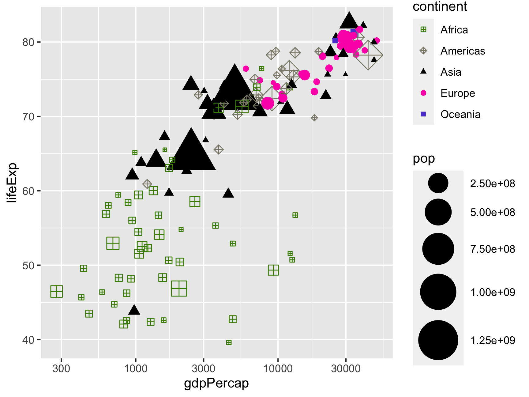
Phew. That’s ugly.
One last thing we can do with scales is format how they show up on the plot. Notice how the population legend uses scientific notation like 2.50e+08. This means you need to move the decimal point 8 places to the right, making it 250000000. Leaving it in scientific notation isn’t great because it makes it really hard to read and interpret.
If you load the scales library (which is installed as part of tidyverse but isn’t automatically loaded), you can use some neat helper functions to reformat the text that shows up in plots. For instance, we can make it so population is formatted as a number with commas every 3 numbers, and the x-axis is formatted as dollars:
library(scales)

ggplot(gapminder_2007,
       aes(x = gdpPercap, y = lifeExp,
           color = continent, shape = continent, size = pop)) +
  geom_point() +
  scale_x_log10(labels = dollar) +
  scale_size_continuous(labels = comma)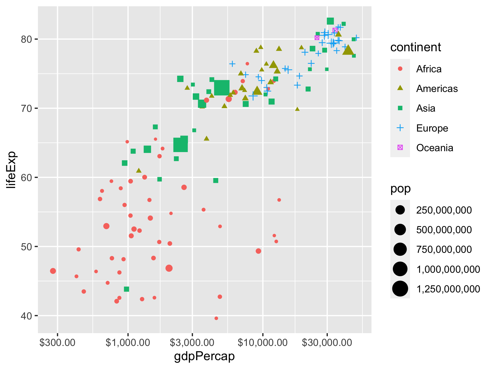
Check the documentation for scales for details about all the labelling functions it has, including dates, percentages, p-values, LaTeX math, etc.